Bayesian Analysis of an A/B Test

Last month I noted that I was looking into Bayesian data analysis to aid better decision-making with marketing data. Well, it's time to start using some software (R) and getting to work.

Links to articles on the advantage of Bayesian data analysis over traditional null-hypothesis significance testing (NHST) were provided in that first post. More good articles can be found on John K. Kruschke's blog.

In a nutshell, on the plus side with Bayesian analysis you can generate richer information about your parameters. And you don't have the  problems of the investigator's intent and the hidden priors of NHST.

The one hitch to Bayesian analysis is that you may have to compute a difficult integral. There are a few techniques to make it doable. First, make the math easier--use conjugate priors and known distributions. Second, numerically approximate the integral; you'll need this especially if your priors can't be adequately expressed with a convenient distribution. This grid approximation won't work, though, if your parameter space gets too large. Then you are on to Markov chain Monte Carlo (MCMC) methods that extend to large parameter spaces.

Over several posts, we'll look at all 3 techniques, even though we can often get away with conjugate priors and convenient math.

For more detail, we're inspired by and playing along with Chapter 8 of Doing Bayesian Data Analysis by John K. Kruschke. We'll just be using a marketing case instead of the ubiquitous coin flips. (The base R scripts used for the below come from the book.)

A lot of digital marketing cases involve two binomial proportions--open rates, click rates, conversion rates. Luckily, these cases can be easy to solve via exact formal analysis. Because the Bernoulli likelihood function has a ready conjugate function for our prior--the beta distribution.

When we're doing an A/B test of two treatments, we're trying to make inferences about two independent proportions. We are talking about the space of the two combined parameters--every combination of Click-through rate A (θ_A) and Click-through rate B (θ_B).

So what are we testing, anyway? Well, earlier this year some of us wanted to test a marketer's practice of sending out self-promotional, announcement emails. Buried in these announcement emails were offers for a white paper--an actually valuable offer. In other words, in order to promote a useful white paper, the marketer is sending a "Come See How Wonderful We Are at XYZ Expo" email. (This can be considered a classic case of going through the marketing motions.) Our hypothesis was that an email directly promoting the white paper would convert better.

So let's get to it.

We need to determine our priors, calculate the likelihood from the data, use Bayes formula to derive the posterior distribution of our parameters (the click-through rates) and then we can compare the underlying rates from A and B. We can do this with an exact analysis using beta distribution priors and Bernoulli likelihoods.

Priors and Likelihoods and Posteriors, Oh My

We're examining a parameter space over θ_A and θ_B. That is the probability p(θ_A, θ_B) over all combinations of θ_A and ϑ_B. In our case, since our channels are independent, p(θ_A, θ_B) = p(θ_A) * p(θ_B). Similarly, our likelihood is a product of two Bernoulli functions. We combine these priors and likelihood functions and, through the magic of beta distros being conjugate to Bernoulli likelihoods, badda bing, badda boom, our posterior is a product of independent beta distributions too.

We have our recipe. Just add some constants, some data, and stir.

Priors

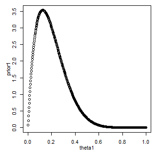
Our historical data shows around a 20% conversion rate for offer emails to this target, so we'll use that in choosing both priors, setting them the same. A beta distribution with a = 2 and b = 8 works nicely.

The prior for B is the same. 

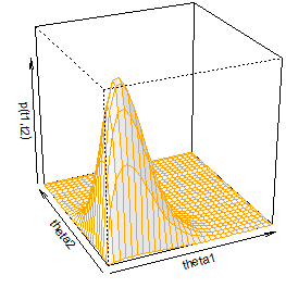
A perspective plot over both parameters looks as follows.

Likelihood

Our likelihood functions are:

θ_A^z_A * (1 - θ_A)^{(N_A - z_A)}

and

θ_B^z_B * (1 - θ_B)^{(N_B - z_B)}

where the z's and N's are the number of hits and sample size, respectively, of each channel, A and B. Here is where our sample data entered the mix.

In our test, A is the group that received the self-promotional email. B is the offer email. Our actual data is:

z_A = 85 ; N_A = 637
z_B = 219 ; N_B = 722

Posterior

Through our "badda-bing" math, we have the product of independent beta distributions as our posterior:

beta(θ_A | z_A + a, N_A - z_A + b), and
beta(θ_B | z_B + a, N_B - z_B + b).

Now we can examine the posterior distribution by evaluating it across the θ_A, θ_B space. Here is the contour plot.

What have we learned?

Looking at this plot we can see that θ_B is very likely greater than θ_A. 

How much greater?

We can sample from the two independent beta distributions of the posterior and compare them. Here we can see the mean of the difference and the 95% HDI (Highest Density Interval) of the difference. The mean and HDI are above zero, leading us to believe that the difference in B over A is real.

That is, the offer email performs better than the self-promotional one. 

Much better.

Conclusion: make your content and your emails for your reader, not about yourself.